Causal Structure Learning

Abstract: Learning cause-effect relationships is a central goal in many research areas. Various techniques and algorithms exist to learn causal structures solely based on observational data as interventions are often infeasible for real-world applications. The PC algorithm is a constraint-based causal structure learning algorithm to learn the underlying causal structure of observed variables by performing conditional independence tests (CI-tests). Motivated by the steady advances in hardware technology, purely CPU- or GPU-based parallel implementations of the PC algorithm such as pcalg and cuPC do not harness the computational power of all processing units available in a heterogeneous setting (having both GPU and CPU).
We therefore focussed on heterogeneous CPU-GPU computing for constraint-based causal structure learning. We evaluated two state-of-the-art implementations of the PC algorithm (i.e. pcalg and cuPC) and derive potential performance improvements by utilizing the available heterogeneous setup. We propose a general approach for heterogeneous constraint-based causal structure learning using static workload-partitioning. The core idea is to perform the CI-tests simultaneously on both CPU and GPU and merge the results afterwards. We provide a reference implementation based on pcalg and cuPC for our heterogeneous approach. Our experimental evaluations show that for large problem sizes the additional overhead of the heterogeneous setting becomes negligible and we achieve comparable performance to modern PC algorithm implementations while utilizing the available resources of both CPU and GPU.
Setting: This project ran as part of a seminar called "Causal Inference – Theory and Applications in Enterprise Computing" during my master's degree at Hasso Plattner Institute, together with Tobias Maltenberger and under the guidance of Christopher Hagedorn and Johannes Huegle.
The ladder of causation
Causality sorts into three kinds of question, a hierarchy Judea Pearl calls the "Ladder of Causation".
-
Rung 1. Association: Asks what we see: what observing X tells us about Y, captured by P(Y|X). It only requires the joint distribution of the observed variables, which can be estimated from observational data.
-
Rung 2. Intervention: Asks what happens if we act: how Y responds when we set X to a value, written P(Y|do(X=x)). This can be answered in two ways. The experimental route is via randomized controlled trial (often infeasible or not ethically justifiable — e.g. randomly assigning people to smoke). The observational route requires the causal graph G together with a set of assumptions (e.g. no unmeasured confounding variables, positivity,...). A causal graphical models (DAG + conditional distributions), is what makes the observational route possible. The graph encodes the influences between the variables and the do-calculus settles the identification question: whether P(Y|do(X=x)) can be written as a functional of the observational distribution, and if so, which one.
-
Rung 3. Counterfactuals: Asks what would have happened otherwise: what Y would have been for this specific unit had X been different, given what we actually observed. This requires the full structural causal model (a DAG with the functional forms and the noise distributions). Each variable is generated by an equation Vᵢ = fᵢ(parents, Uᵢ), where the noise term Uᵢ captures everything specific to a unit that the model does not explain. Abduction, action and prediction then turn this into a procedure: given the evidence about a specific unit, what would Y have been had X been different, i.e. P(Y_x | X = x', Y = y')?
This splits the field in two: statistical inference lives on rung 1 and answers questions about the world as it is, while causal inference lives on rungs 2 and 3 and answers questions about a world we change or a world that might have been.
Learning a causal structure from data
A causal graphical model represents causal relationships as a directed acyclic graph (DAG): every node is a random variable, and a directed edge from one node to another means the first random variable is a direct cause of the second random variable. Causal structure learning is the task of recovering that graph from data.
Constraint-based algorithms do it by elimination. They start from a fully connected graph and ask, for pairs of variables, whether the two are statistically independent once some set of other variables is accounted for — a conditional independence test, or CI-test. If they are, the edge between them cannot represent a direct cause and gets removed. What remains after all tests is the undirected skeleton of the graph; a second step then orients the remaining edges by repeatedly applying deterministic rules.
Constraint-based causal structure learning rests on three assumptions:
- Causal Markov condition: G and P satisfy the causal Markov condition if and only if a node of G is independent of all of its non-descendants given all its parents.
- Causal faithfulness condition: G and P satisfy the causal faithfulness condition if and only if conditional independence is only implied by the causal Markov condition.
- Causal sufficiency condition: Causal sufficiency holds if all common causes of the observed variables are included in the data.
The Markov condition states that every conditional independence entailed by G holds in P; faithfulness states the converse. Together, the two conditions make the conditional independence in P exactly those entailed by G, which is why the absence of an edge can be inferred from a CI-test. Under these assumptions, the CI-tests identify the Markov equivalence class of the true DAG and not the DAG itself.
The PC algorithm is the best-known algorithm of this family. Its first phase, the adjacency search, is organized in levels: at level l, independence is tested conditioned on separation sets of size l. Level 0 asks for plain (unconditional) independence (i.e. whether two variables are independent without conditioning on anything - X ⫫ Y ), level 1 conditions on a single other variable (X ⫫ Y | Z,), and so on. After every level, the edges found to be independent are dropped, which shrinks the work for all following levels.
Two properties matter for what we worked on. First, the adjacency search dominates the runtime almost entirely — the orientation phase is cheap by comparison, which is why every optimization effort targets the search. Second, the original PC algorithm is order-dependent: the result depends on the order in which the variables happen to be given, which rules out parallel execution. PC-stable (Colombo & Maathuis, 2014) fixes this by introducing an order-independent variant of the PC algorithm, making edge removals within a level invisible to the other tests in that same level, and that order independence is what makes the whole thing parallelizable in the first place.
Two parallel implementations define the state of the art here:
- pcalg (Kalisch et al., 2012) is the reference implementation of the PC algorithm and the package most causal discovery work builds on — an R package with a C++ core, which runs the CI-tests of a level in parallel across all CPU cores using OpenMP. The implementation can be found on CRAN.
- cuPC (Zarebavani et al., 2019) is the fastest published implementation and implements PC-stable in CUDA for the GPU. It adds a set of GPU-specific optimizations — compacting the adjacency matrix between levels, sharing results between tests with a common separation set, keeping hot data in shared memory, and stopping other threads early once an edge has been removed — which together make it orders of magnitude faster than pcalg. The source is on GitHub.
Heterogeneous computing - challenges and opportunities
CPUs are optimized for efficient sequential code execution (through branch prediction, deep cache hierarchies, and speculative execution). GPUs are optimized for highly parallel arithmetic operations on hundreds or thousands of cores. Heterogeneous computing is the idea of using both Processing Units (PU) at the same time instead of focussing on one. In a GPU-accelerated program, the CPU usually sits idle other than to launch kernels.
However, introducing another PU as additional computing resources poses several challenges: workload must be partitioned, tasks need to be scheduled between the two PUs, and the results need to be synchronized afterwards. This leads to an organizational effort for cooperative problem solving and transfer overhead between the two PUs. Partitioning strategies in a heterogeneous setting can be classified into static and dynamic.
- Static workload partitioning: A static partitioning-strategy fixes the mapping of tasks to the specific PU prior to the program execution and is indifferent to the hardware-specific capabilities. A static strategy introduces little overhead but is prone to load imbalance (as for example edge removals are not evenly distributed across partitions which leads to load imbalance).
- Dynamic workload partitioning: A dynamic rationing strategy implies dynamic changes during runtime which incurs more overhead but can handle a potential load imbalance.
In the context of constraint-based causal structure learning, partitioning can happen at vertex-level (all CI-tests for all edges of one variable are assigned to one PU), at edge-level (all CI-tests for one edge are assigned to one PU) or at CI-test-level (CI tests for a single edge are spread across PUs).
Runtime characteristics of the adjacency search
Before partitioning the workload, we characterized how the runtime of the adjacency search is distributed. We took cuPC as the baseline, since it is the faster of the two implementations, generated synthetic data with randomDAG() from pcalg so that the ground-truth graph was known, and varied the parameters one at a time.
Three parameters drive the runtime up sharply: the number of variables n, the edge probability p of the underlying graph, and the significance level α. A larger α removes fewer edges in the early levels and therefore leaves more tests for the later ones. The number of samples m has little influence, because the CI-test for multivariate normal data is computed on the correlation matrix and not on the samples themselves.
The distribution across the levels matters more. The number of CI-tests peaks at levels 1 and 2, and these two levels account for more than 90% of the total runtime.
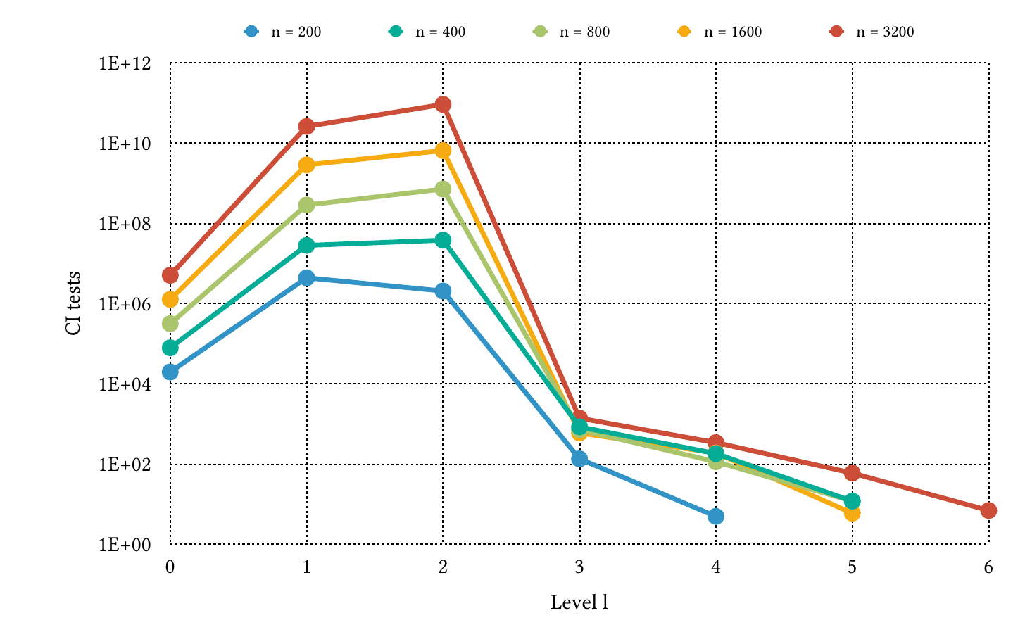
We then measured the GPU's utilization per level via the sm_efficiency metric of nvprof. cuPC uses a separate CUDA kernel per level, so the per-level measurement needs no further instrumentation:
| Level l | n = 200 | n = 400 | n = 800 | n = 1600 | n = 3200 |
|---|---|---|---|---|---|
| 0 | 16.75% | 36.34% | 74.33% | 90.87% | 97.46% |
| 1 | 90.52% | 90.45% | 91.55% | 94.45% | 98.92% |
| 2 | 45.96% | 51.69% | 36.91% | 35.83% | 100.00% |
| 3 | 22.16% | 29.07% | 34.89% | 35.52% | 49.49% |
| 4 | 2.92% | 12.80% | 16.04% | 14.79% | 28.94% |
| 5 | – | 3.54% | 4.73% | 5.73% | 13.49% |
| 6 | – | – | – | – | 9.35% |
GPU utilization per level (m = 6400, p = 0.2, α = 0.05). Bold marks utilization above 90%.
From 1,600 variables on, the first three levels saturate the GPU, and at 3,200 variables level 2 reaches full utilization. For the same runs, top and mpstat show the CPU sits idle. One PU is saturated while the other is unused, and this happens on the levels that account for most of the runtime. This marks the motivation for our heterogeneous approach.
Partitioning the adjacency search across both PUs
The approach we propose runs a subset of each level's CI-tests on the GPU and the remaining ones on the CPU, simultaneously.
We partition at vertex-level using a static approach. Spreading the CI-tests for a single edge across both PUs would introduce the overhead cuPC already describes for parallelization within an edge: redundant tests and synchronization inside what should be one unit of work. Since the approach targets large graphs (from roughly 1,600 variables onwards), the vertex-level partitions are small enough to balance.
The partitioning factor pf controls the share of vertices assigned to the CPU. The first n × pf rows and columns of the adjacency matrix are tested on the CPU, the remaining n × (1 − pf) on the GPU. pf is fixed prior to execution and stays constant across all levels.
Each level then runs in three phases:
- Partition the CI-tests at vertex level according to pf.
- Execute them simultaneously on both PUs, each one working on its own submatrix and parallelizing internally across its own cores.
- Merge the two partially updated submatrices back into one adjacency matrix before the next level starts.
Implementation
The reference implementation combines the two existing implementations. We extracted the adjacency search and the CI-test from pcalg's C++ core, removed its R bindings, and embedded the result into cuPC's CUDA sources. The code can be found on GitHub.
Four implementation details are worth noting:
Memory. On the CPU side, the graph is held in a Boost Graph Library (a well-established C++ library providing both data structures and frequently used graph algorithms) structure. On the GPU side, data used only by the GPU (the separation sets and the bookkeeping for edge orientation) is allocated with cudaMalloc, while the GPU's graph representation uses cudaMallocManaged. Managed memory places the graph in an address space both PUs can access directly and, through demand paging, transfers only the pages that changed. Benchmarking the alternative (plain cudaMalloc plus explicit cudaMemcpy into a host buffer and back) showed a negligible difference for large n, so we kept the managed variant for the better programming experience.
Merging only the differences. Reads and writes into managed GPU memory from the host thread are expensive, so the merge phase propagates only the edges that were added (level 0) or deleted (all later levels) instead of copying whole submatrices. In the levels that remove few edges, the merge is therefore nearly free.
Keeping all CPU threads busy. The CPU thread collects the edges in its share and runs their CI-tests in parallel with OpenMP across t threads, where t is roughly the core count. In the higher levels, the number of remaining edges k can drop below t, which would leave threads idle. For that case we added a second layer of parallelism using Armadillo (the scientific C++ library for performing the CI-tests on the CPU side), so that the CI-tests for a single edge are spread across the remaining threads.
Comparability. pcalg and cuPC perform CI-tests with different criteria - to ensure that the two halves of the same level applied the same criteria, we modified the CPU-side implementation. pcalg compares Fisher's z-transformed partial correlation against the significance level α directly, while cuPC derives a per-level threshold τ from it.
Results
All measurements ran on a bare-metal server with two Intel Xeon Gold 6148 CPUs (20 cores each, 2 threads per core) and 750 GB of RAM, plus four NVIDIA Tesla V100-SXM2 GPUs with 32 GB of high-bandwidth memory, connected over PCIe Generation 3. Every experiment was repeated 100 times and averaged.
The overhead the approach introduces consists of the CPU-side memory allocation, the final transfer back to R, and one merge phase per level. All three grow linearly with the number of variables, while the cost of the CI-tests grows far faster. The overhead should therefore lose relevance as the problem size increases:
| Variables n | Heterogeneous [s] | cuPC [s] | Difference |
|---|---|---|---|
| 1600 | 3.29 | 1.82 | 80.53% |
| 1800 | 4.62 | 2.64 | 74.66% |
| 2000 | 5.91 | 3.62 | 63.06% |
| 2200 | 8.50 | 5.56 | 52.79% |
| 2400 | 19.35 | 15.22 | 27.14% |
| 2600 | 18.68 | 13.96 | 33.85% |
| 2800 | 24.46 | 18.97 | 28.93% |
| 3000 | 47.93 | 39.50 | 21.36% |
| 3200 | 43.72 | 34.97 | 25.02% |
Total runtime against cuPC (m = 6400, p = 0.2, α = 0.05, pf = 0.05). The difference is the additional runtime of the heterogeneous version relative to cuPC. Each row uses its own randomDAG() draw, which is why the runtimes are not strictly monotonic in n. We do not compare against pcalg, which is orders of magnitude slower than cuPC.
At 1,600 variables the heterogeneous version needs 80% more runtime than cuPC, almost all of it merge overhead. At 3,200 variables the difference is down to 25%. The heterogeneous version stays slower than cuPC over the whole range we measured, but the gap narrows as the problem size grows, which is what the linear overhead predicts. At the upper end the approach reaches comparable performance to a pure-GPU run while part of the work runs on a PU that was previously idle.
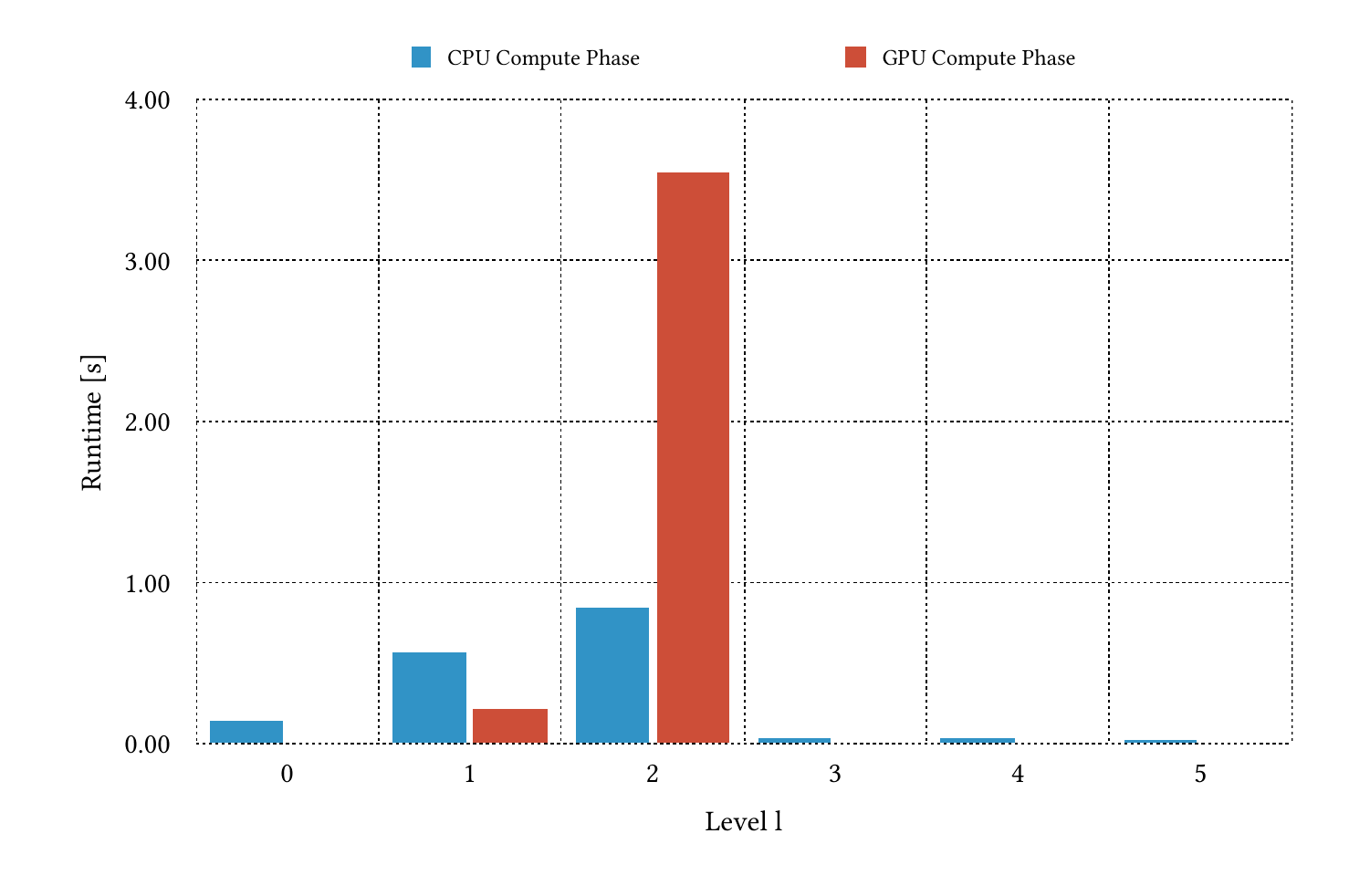
The main limitation is the static workload partitioning strategy & the corresponding fixed factor. Measured per level at pf = 0.09, the two PUs are mismatched in opposite directions depending on the level. Level 0 consists of a large number of independent CI-tests without synchronization in between and is therefore well suited to the GPU, so pf = 0.09 assigns the CPU more work than it can keep up with. At level 1 the CPU is the slower of the two and the GPU waits. At level 2, with the same factor, the GPU needs 3.54 seconds against 0.84 seconds on the CPU. A single constant cannot fit all levels: the cost of a CI-test differs per level, and edge removals are not evenly distributed across the two partitions, so some load imbalance remains.
Discussion and future work
Our experimental evaluation of the proposed approach proves the feasibility of the heterogeneous algorithm for performing the adjacency search of causal structure learning. We also achieve comparable performance to the original implementation of cuPC.
The next step is a dynamic partitioning strategy that recomputes the factor per level from the cost of a CI-test at that level, the relative compute power of the two PUs, the interconnect between them, and the skew in edge removals. Two smaller extensions: running individual levels exclusively on one PU, which should pay off for the late levels, where so few CI-tests remain that the merge phase costs more than the split saves; and setting CUDA block sizes per level instead of keeping cuPC's static ones, to reduce idle time in underutilized kernel threads.
Paper: The approach, the measurements, and the theoretical background and related work in full detail can be found in the paper written as the final deliverable of the seminar, together with Tobias Maltenberger: Heterogeneous Computing for Constraint-based Causal Structure Learning (PDF).