Histopathologic Cancer Detection

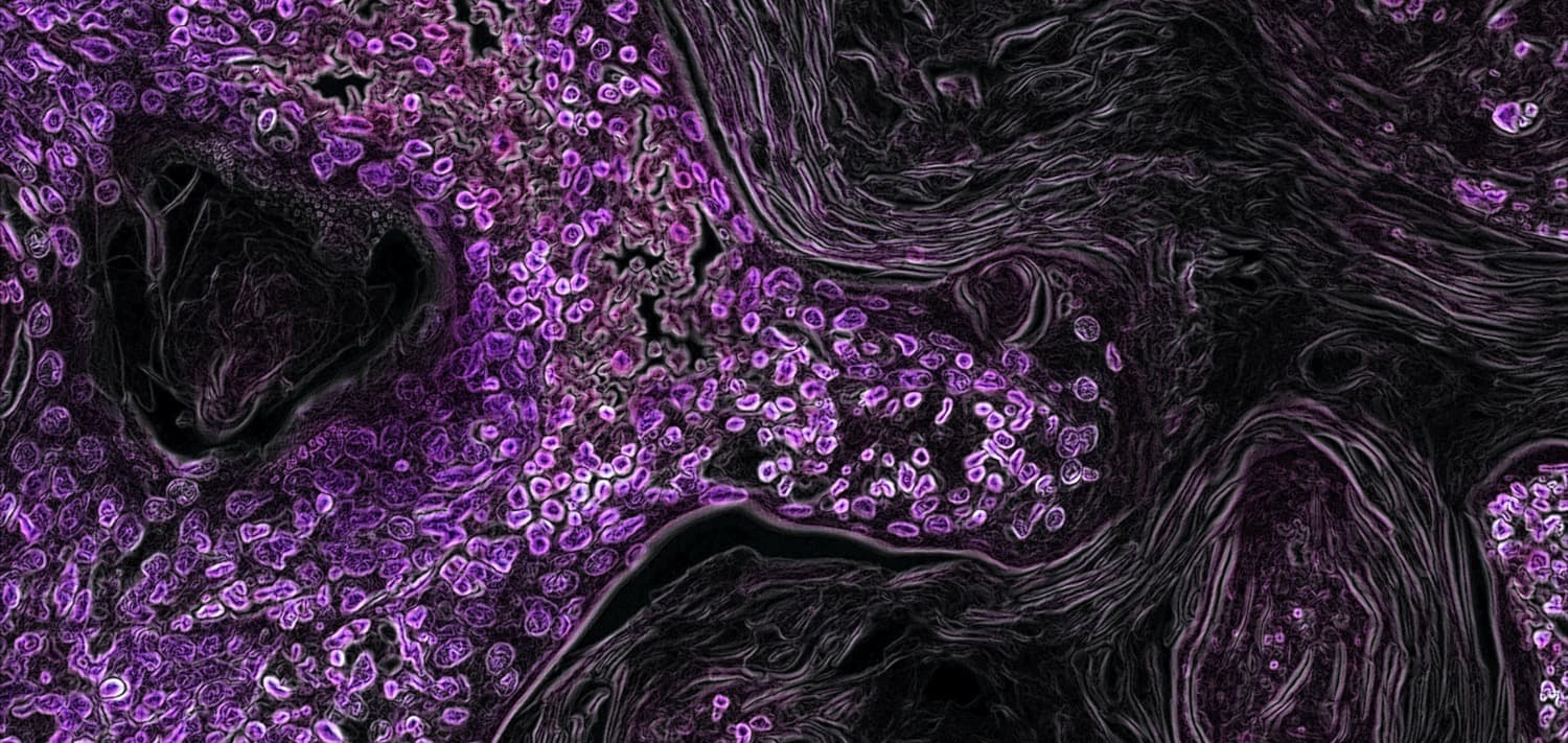
Abstract: Whether a lymph node contains metastatic tissue determines how a cancer is staged, and consequently how it is treated. Answering that question means examining the lymph node under a microscope, section by section. We evaluated six Deep Learning architectures on the same 220,025 tissue patches from lymph node sections (the PCam dataset), measuring how reliably they separate malignant from non-malignant tissue. The best model, a pretrained ResNet34, reached 99.53% AUROC, a metric that, unlike accuracy, is robust to unbalanced classes and independent of the decision threshold. Stain normalization, the standard preprocessing step for this kind of data, did not help: it made the results worse on almost every model.

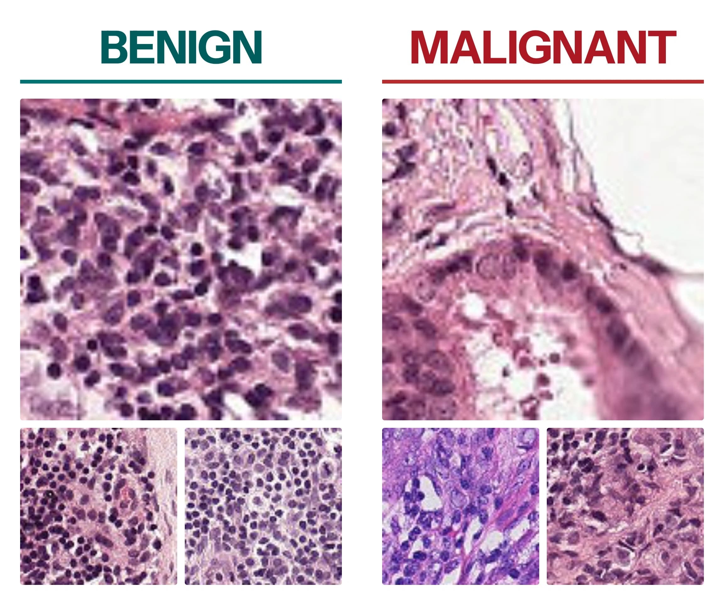
Six stained lymph node tissue patches, three labelled benign on the left and three labelled malignant on the right. The benign ones show small, evenly sized dark nuclei; the malignant ones show larger cells of varying size, grouped into clusters and streaked with pink fibrous tissue. — Six 96×96 px patches from the PCam dataset. A patch counts as malignant if its centre 32×32 px region contains tumour tissue.

Differentiation of malignant vs. benign samples: Pathologists differentiate malignant vs. benign tissue by mulitple aspects. The first is uniformity: a benign node is a monotonous collection of small lymphocytes whose nuclei are all roughly the same size and shape, while metastatic cells stand out as noticeably larger, with more pale cytoplasm and with nuclei that vary from cell to cell. The second is arrangement: tumour cells group into nests, cords or gland-like structures and often pull a pink fibrous stroma along with them, instead of spreading out evenly like the lymphocytes around them.

Context: Mortality rates associated with cancer in Germany have been steadily declining since the 1990s. However, the absolute number of new cases has almost doubled since the 1970s due to an increased overall life expectancy and an aging population. In 2016, there were 229,900 new cancer diagnoses in Germany, and 791,770 people were living with a diagnosis made within the previous five years (Bericht zum Krebsgeschehen in Deutschland 2016).

Even at an early stage, tumors frequently spread from the primary tumor into the surrounding lymph nodes and form metastases. That shifts the prognosis sharply: the 5-year survival rate falls from 82.5% at stage II, without lymph node metastases, to 59.5% at stage III, with them (O'Connell et al.). Finding those deposits means working through a sentinel lymph node section by section, and in 60–70% of cases the pathologist goes through all of it to find nothing at all (Litjens et al.).

Setting: This project ran as part of a seminar called "Deep Learning" during my master's degree at Hasso Plattner Institute, together with Eric Fischer, Nicolas Alder, Erik Langenhan, Simon Witzke, and Nathaniel Müller.

What we compared: Deep Convolutional Neural Networks (CNNs) now reach accuracies comparable to medical professionals (Han et al., Coudray et al.), and studies have found that pathologists working with a Deep-Learning assistant detect more, and faster (Steiner et al., Kiani et al.). The Deep Learning architecture is critical to reaching those accuracies, yet most research papers report only the one that happened to work best on their own data. So we put six different approaches to the test on the same dataset, under the same conditions, and further compared whether pretraining on ImageNet helps, and whether stain normalization does.

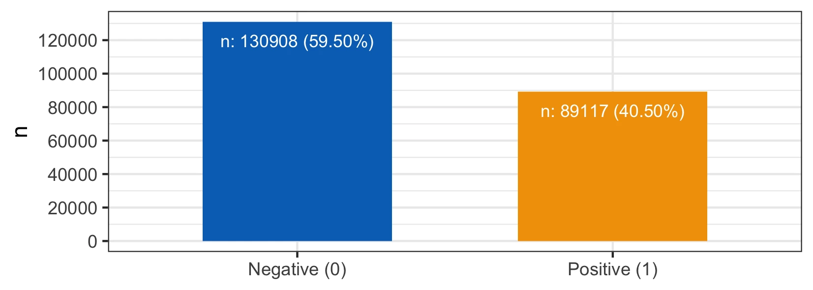
Dataset: We utilized a slightly modified version of the PCam dataset, which was also used for a Kaggle competition. This dataset consists of 220,025 images of tissue from lymph node sections, 96x96 pixels, and 27,935 bytes each. Of these pictures, 130,908 show no signs of cancer (class 0), while the other 89,117 pictures show signs of cancer (class 1).

Bar chart of the label distribution: 130,908 negative patches (59.50%) against 89,117 positive ones (40.50%)

Stain Normalization: In the process of deriving the sample tissues, the hematoxylin and eosin (H&E)-staining was used to analyze different biological substances with different selective affinities. The stained slides are analyzed using a microscope while being illuminated from below. The stain vector is the proportion of each wavelength absorbed by the stained slide. This stain vector can vary between the different stains used in the process, but it can also vary considerably for the same stain depending on factors such as the manufacturer, storage conditions before use, and the application method itself.

As the stains might originate from different laboratories and different preparation methods, systematic biases are likely. In order to account for the inconsistencies in the preparation of histology slides, we applied staining normalization.

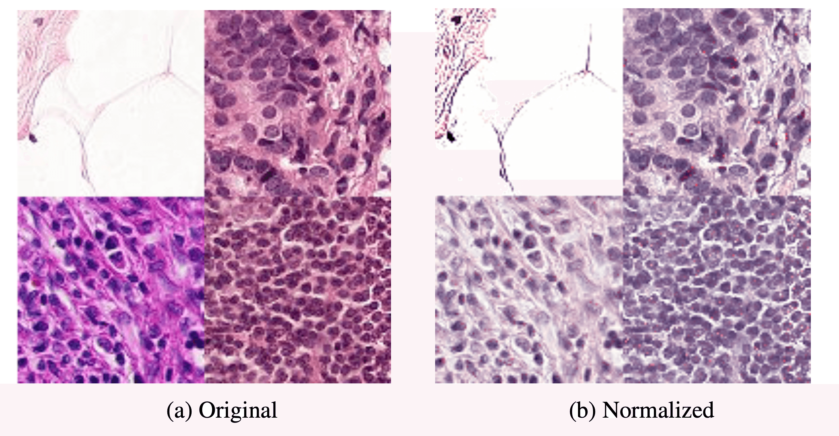
Normalized vs. non-normalized tissue slide pictures

We pursued the approach of Macenko et al. and their SVD-geodesic method for obtaining normalized stain vectors. The normalization was done before loading the images. This procedure was chosen to reduce the image-loading time as normalizing all images in the dataset required multiple hours. As part of the normalization algorithms, the eigenvalues of the stain-value-matrices were computed - however for some matrices, the eigenvalue-decomposition did not converge. As this only accounted for 418 out of 220,025 pictures, we did not include these pictures in the normalized dataset.

For the normalization we used and modified an existing Python implementation of the method proposed by Macenko et al.

Architectures: We evaluated six Deep Learning architectures on the dataset: VGGNet11, VGGNet19, ResNet18, ResNet152, DenseNet121, and DenseNet201. In addition, we compared pretrained variants: DenseNet121, DenseNet201, ResNet34 and ResNet101.

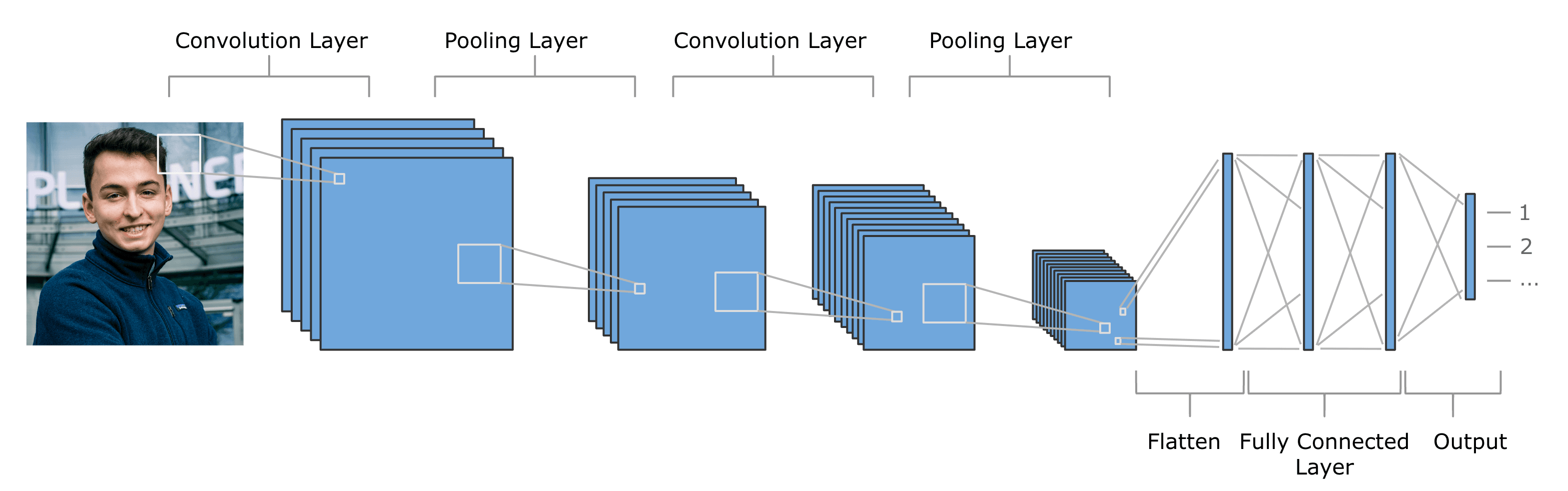
We also ran a LeNet5 as a deliberately simple baseline. It never got past 59.09% accuracy (exactly the share of the majority class) - so it effectively did not learn anything and we excluded it from the analysis.

Experiment setup: We split the data into 176,020 training images (80%) and 44,005 test images (20%), about 6 GB in total, and skipped cross-validation: at this size a pure train-test split is enough, and k-fold cross-validation would have multiplied the training time. The models are PyTorch architectures wrapped in skorch, with the classification layer adjusted to a single output. In total we ran 150 experiments over 30 epochs, with binary cross-entropy logit loss and an Adam optimizer, batch size 128 and a learning rate of 0.01. The VGGNets needed 0.001 and an Adamax optimizer to produce usable results. Training was conducted on Google Colab (Nvidia Tesla K80) and on a server we had access to as part of the research group at our university with four Nvidia Tesla V100 GPUs. Every run was logged in Neptune.ai project, so each model run stayed reproducible and could be pulled back out for prediction. The code for our project can be found on GitHub.

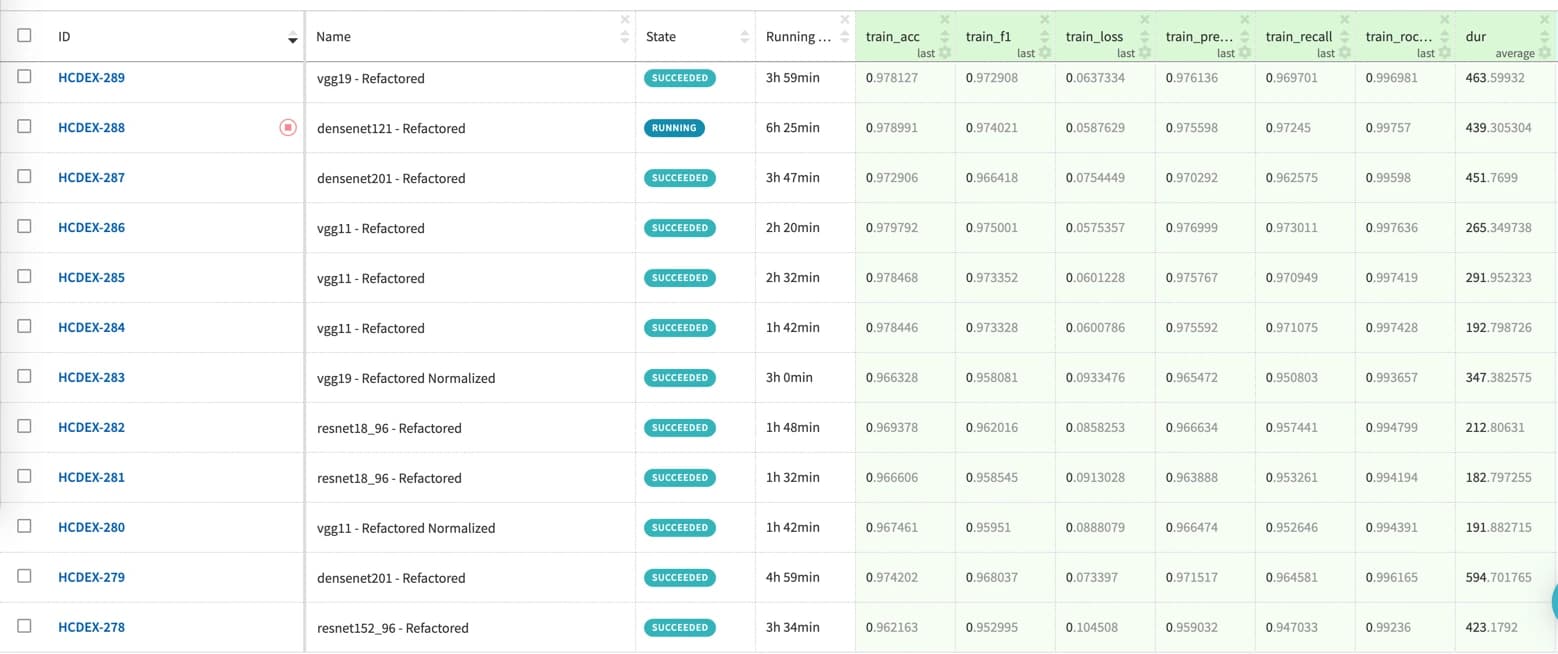
Table of experiment runs in Neptune with accuracy, F1, loss, precision, recall and AUROC per run

Every experiment run with its metrics in Neptune.ai.

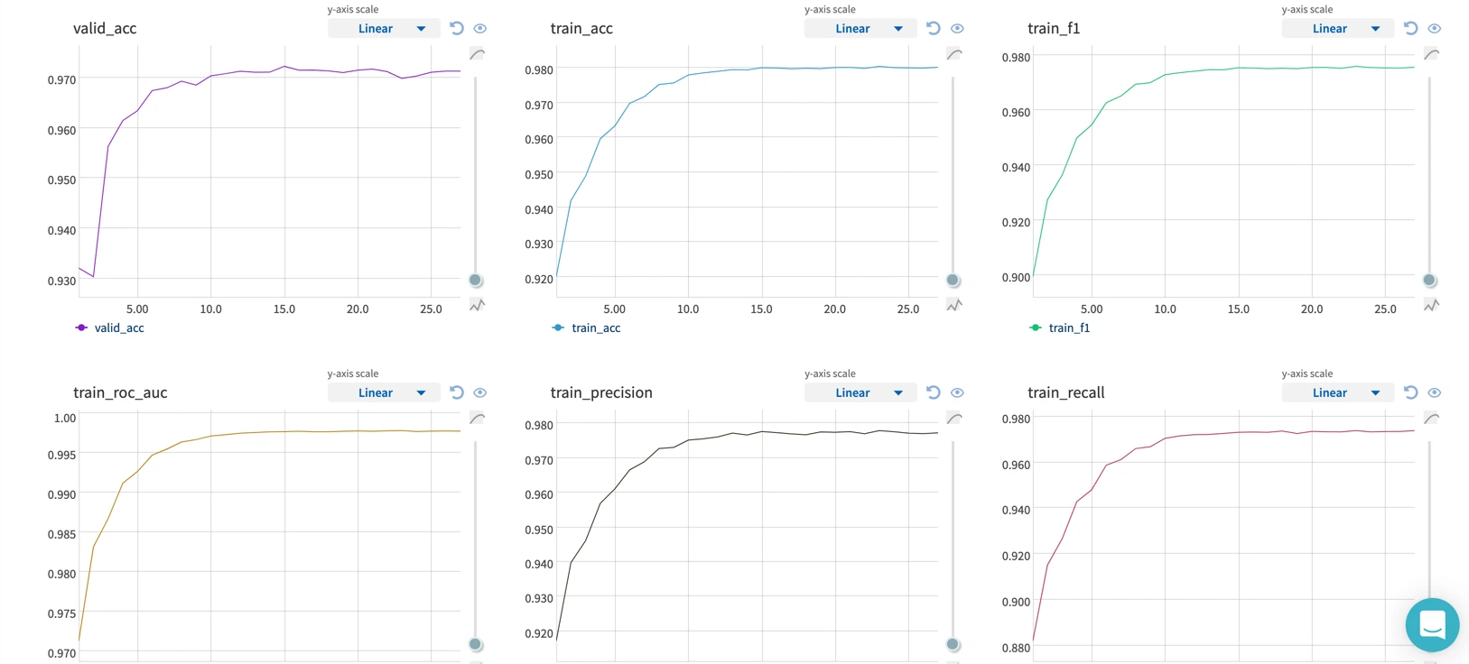
Six metric curves from a single run in Neptune: validation accuracy, training accuracy, F1, AUROC, precision and recall over 30 epochs

Training and test accuracy curves across multiple epochs.

Results: On the non-normalized full dataset, a non-pretrained DenseNet201 gave the best accuracy (97.65%) and F1 (97.09%). The best recall (97.57%) came from a second DenseNet201 run, the best AUROC of 99.53% from a pretrained ResNet34.

Metric	DenseNet201	DenseNet121	DenseNet201 (second run)	ResNet34 (pretrained)
Test accuracy	97.65	97.47	97.19	97.11
Test F1	97.09	96.85	96.57	96.43
Test precision	97.28	97.47	95.58	96.45
Test recall	96.91	96.24	97.57	96.41
Test AUROC	97.54	97.27	97.25	99.53

Three things surprised us. Depth of the networks we used barely mattered: VGGNet19 gained almost nothing over VGGNet11, and the same holds for ResNet18 against ResNet152 and DenseNet121 against DenseNet201. Pretraining had a negligible effect, about 1% better for ResNets, about 1–2% worse for DenseNets. And normalization made things worse against our expectation on almost every model. Why is hard to say with a black-box model: it may be that the networks key on colour and contrast more than we assumed, and that normalization removed relevant signal along with the noise.

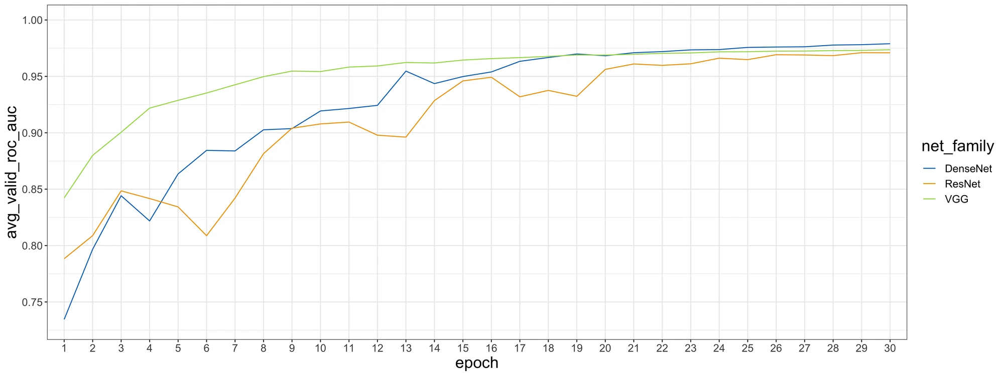
Weighted mean validation AUROC over 30 epochs for the three network families: VGG rises fastest, DenseNet and ResNet catch up by epoch 20

Averaged over all runs per family. VGG climbs fastest, but after roughly 20 epochs the three are indistinguishable.

What we would take into clinical practice: For a dataset of this size, VGGNets, ResNets, and DenseNets are all reasonable choices; with a smaller one, DenseNet201 is the better pick

Future work: An interesting aspect one can further investigate is performing stain split. Beyond colour normalization, the Macenko deconvolution decomposes the image into its two constituent stains, which encode complementary information. Hematoxylin binds to cell nuclei (blue-purple), whereas eosin binds to cytoplasm and connective tissue (pink). The resulting channels therefore separate nuclear morphology from the surrounding tissue context.

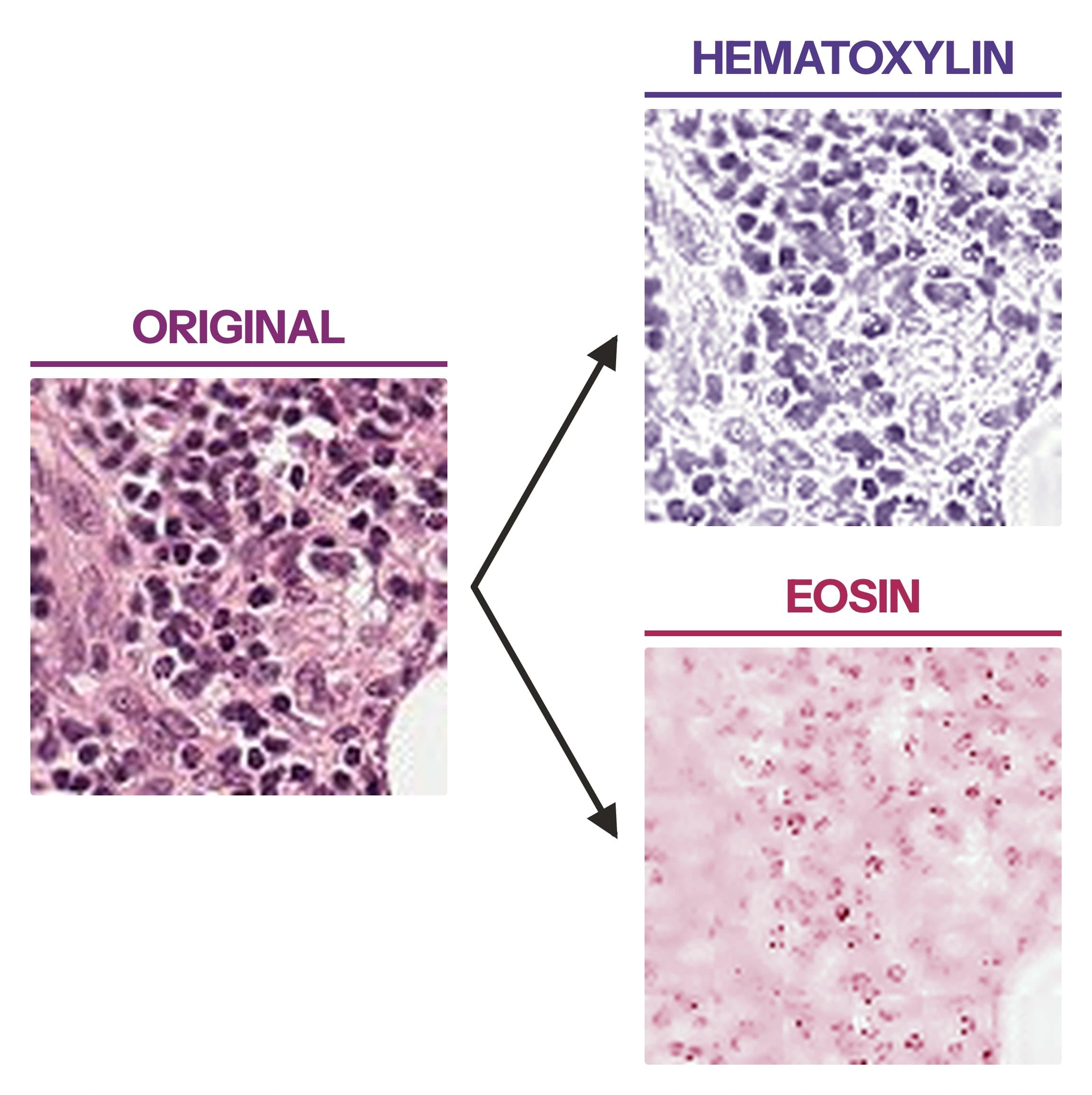
One stained tissue patch with two arrows pointing to its separated channels: a purple hematoxylin channel showing only cell nuclei, and a pink eosin channel showing only cytoplasm and connective tissue. — Unmixing a patch into its hematoxylin and eosin channels, an intermediate step of the Macenko normalization.

The approaches we took only worked with normalized, but not split lymph node tissue slides. Feeding both channels into a Deep Learning Network separately hands the model the nuclear morphology as its own signal, the very cue a pathologist reads, instead of flattening the colour variation away. Given that normalization cost us accuracy rather than improving it, that looks like a promising direction. Chakraborty et al. report promising results for exactly that combination on a breast cancer dataset, pairing stain decomposition with a dual-channel residual network.

Paper: Looking back, this research project was a pleasure to work on. The full paper, written as the final deliverable of the seminar, can be found here: Deep Learning for Histopathologic Cancer Detection (PDF).